Your team just hit VRAM OOM during a demo prep run. The A100 40GB you provisioned for a Llama-3-70B deployment looked fine on paper until the KV cache ballooned at 8K context. You could throw two H100s at it and move on, or you could run the 30 seconds of arithmetic you skipped before provisioning.
Four decisions separate teams that run GPUs above 70% utilization from those idling at 35% while paying full price: workload classification, VRAM calculation, instance selection, and pricing model alignment. Get any of them wrong and you’ll either hit a production ceiling or burn budget on capacity you can’t fill. Once all four are locked in, deployment is the execution step that wires them together.
Start with your workload class, not the GPU spec sheet
The first decision is workload classification, because training, fine-tuning, and inference each have a distinct compute signature that points toward different hardware.
Full training demands sustained throughput over hours or days. Your GPU spends most of its time executing Allreduce across data-parallel replicas and moving optimizer states between High-Bandwidth Memory (HBM) and compute units. Memory capacity bounds the maximum batch size per device, and memory bandwidth determines how fast weight updates move. A model trained with AdamW in mixed precision stores weights, gradients, first moments, and second moments, totaling 16-18 bytes per parameter depending on whether gradients are stored in FP16 or FP32. That math makes VRAM the primary scaling constraint.
Fine-tuning with LoRA reshapes the memory profile. It freezes the base model weights and trains low-rank decomposition matrices. With rank=16 on Llama-3-7B, you’re training roughly 4.2 million parameters instead of 7 billion. The base model stays in BF16 (or FP16) on-device, the LoRA adapters are negligible in size, and AdamW optimizer states only cover the trainable parameters. Total VRAM drops to around 18GB for a 7B model, which fits on a single A100 80GB with room for activations during the forward pass. Runpod’s LLM fine-tuning GPU guide covers this workload class in depth.
Inference splits into two optimization targets. Batch inference maximizes throughput per dollar by packing more sequences into each forward pass and tolerating the latency required to fill that batch. Real-time inference optimizes for TTFT (time-to-first-token), which is FLOPS-limited during the prefill phase. Inter-token latency in the decode phase scales with memory bandwidth. An H100 SXM’s 3.35 TB/s HBM3 bandwidth serves tokens faster than an A100’s 2.0 TB/s because decode is memory-bound once the KV cache is populated, and the KV cache grows with both sequence length and batch size.
Data modality shapes GPU choice too. LLMs are KV-cache-bound and their VRAM requirements scale with context length. Diffusion models like SDXL are VRAM-sensitive to resolution and batch size, with relatively modest parameter counts (the SDXL base model sits at approximately 3.5B parameters across UNet and VAE; the refiner adds a further 6.6B if the full pipeline is intended). Multimodal models like LLaVA combine both the KV-cache growth of LLMs and the resolution-driven VRAM sensitivity of diffusion models: the vision encoder processes image embeddings that inflate the effective sequence length before the language model ever sees the input, so you’ll hit VRAM limits at batch sizes that would serve a same-size pure-LLM without issue.
Calculate your VRAM before you provision
The inference VRAM formula is:
VRAM = (N_params x bytes_per_param) + KV_cache_size + framework overhead (10-15%)
The KV cache size formula is:
KV_cache_size = 2 x num_layers x num_heads x head_dim x seq_len x batch_size x bytes_per_element
Note that num_heads for GQA models refers to the KV head count, not the query head count (e.g., 8 for Llama-3-70B, not 64). You can find num_layers, num_heads (as num_key_value_heads), and head_dim in the model’s config.json on HuggingFace Hub.
Example for Llama-3-70B at 4K context, batch size 8:
- Weights at BF16: 70B x 2 bytes = 140GB
- Weights at INT4 via bitsandbytes: 70B x 0.5 bytes = 35GB
- KV cache at BF16: 2 x 80 layers x 8 KV heads x 128 head_dim x 4096 tokens x 8 batch x 2 bytes = approximately 10.7GB
- Framework overhead at BF16: 140GB x 0.12 = approximately 17GB
- Total at BF16: approximately 168GB (requires 2x H100 80GB or more with tensor parallelism)
- Total at INT4: approximately 35GB + 10.7GB KV cache + 5GB overhead = approximately 51GB (fits one A100 80GB)
The table below gives you the minimum per-precision VRAM numbers for LLM inference. All values include approximately 12% framework overhead. KV cache is excluded because it varies with sequence length and batch size, so add 2-10GB for typical serving configurations, or significantly more for long-context (8K+) or high-concurrency deployments.
| Model Size | FP16/BF16 | INT8 | INT4 | Min Instance (FP16) | Min Instance (INT4) |
|---|---|---|---|---|---|
| 7B | ~16GB | ~8GB | ~5GB | A100 40GB | RTX 4090 24GB |
| 13B | ~28GB | ~14GB | ~8GB | A100 40GB | RTX 4090 24GB |
| 34B | ~70GB | ~38GB | ~19GB | A100 80GB | A100 40GB |
| 70B | ~145GB | ~73GB | ~40GB | 2x A100 80GB | A100 80GB |
These values cover inference weight loading only. If you’re fine-tuning instead, the numbers shift: full AdamW mixed-precision training multiplies FP16 weight VRAM by 8x, while LoRA at rank=16 adds only about 4GB of combined overhead (activations, intermediate gradients, and optimizer states) on top of the frozen base model. Adjusting rank scales that overhead roughly linearly: rank=8 halves it with some quality cost, rank=32 doubles it for more expressivity.
Here’s where that 8x multiplier comes from. AdamW in mixed precision stores five components per parameter:
- 2 bytes (FP16 weights)
- 2 bytes (FP16 gradients)
- 4 bytes (FP32 master weights)
- 4 bytes (FP32 first moment)
- 4 bytes (FP32 second moment)
That totals 16 bytes per parameter (18 bytes if your implementation keeps FP32 gradients separately). For a 7B model: 7B x 16 = 112GB minimum, which exceeds a single A100 80GB. This is exactly why LoRA’s reduction to approximately 4.2M trainable parameters at rank=16 makes single-GPU fine-tuning viable.
With your VRAM requirements calculated, the next step is matching them to actual hardware.
Match GPU architecture to your workload class
Hardware specs differ enough across current GPU options that a poor choice creates production constraints you can’t optimize away.
| GPU | VRAM | Memory BW | BF16 TFLOPS | Multi-GPU Link | Ideal Workload |
|---|---|---|---|---|---|
| H100 SXM 80GB | 80GB HBM3 | 3.35 TB/s | 989 | NVLink 4.0 (900 GB/s) | Large model training, high-concurrency inference |
| A100 80GB SXM | 80GB HBM2e | 2.0 TB/s | ~312 | NVLink 3.0 (600 GB/s) | Multi-GPU training, 34B+ inference |
| A100 80GB PCIe | 80GB HBM2e | 1.6 TB/s | ~312 | PCIe 4.0 (64 GB/s) | Single-card inference, LoRA fine-tuning |
| L40S 48GB | 48GB GDDR6 | 864 GB/s | ~362 | PCIe 4.0 (64 GB/s) | Diffusion + LLM combo inference |
| RTX 4090 24GB | 24GB GDDR6X | 1.0 TB/s | ~82.6 | PCIe 4.0 (64 GB/s) | Prototyping, quantized 7B-13B |
| AMD MI300X | 192GB HBM3 | 5.3 TB/s | ~1307 | Infinity Fabric (XGMI) | 70B+ BF16 single-card serving |
The H100 SXM 80GB earns its price premium on any workload where inter-GPU communication overhead would otherwise constrain you. NVLink 4.0 delivers 900 GB/s bidirectional bandwidth within a node, providing up to approximately 14x the raw bandwidth of PCIe 4.0, translating to substantially faster Allreduce operations across eight GPUs. Run a 70B-parameter model with tensor parallelism across four H100s and you’re moving approximately 140GB of model weights plus KV cache shards between GPUs on every forward pass. NVLink absorbs that communication cost, while PCIe 4.0 at 64 GB/s turns inter-GPU transfers into the forward pass bottleneck.
The A100 80GB comes in PCIe and SXM variants. The PCIe variant delivers 1.6 TB/s memory bandwidth versus the SXM’s 2.0 TB/s, a ~23% gap that matters for memory-bound serving workloads. The PCIe variant runs 20-30% cheaper and is the right choice for single-card inference on models up to 34B at INT8 and for LoRA fine-tuning of 7B-13B models. The SXM variant justifies its premium when you’re running multi-GPU training where NVLink 3.0 (600 GB/s) provides a 9.4x bandwidth advantage over PCIe 4.0 at scale.
GDDR6 memory on the L40S delivers 864 GB/s bandwidth, which puts LLM inference throughput below an A100 80GB for models heavily bound by memory bandwidth. The Ada Lovelace rasterization silicon on the L40S makes it the right pick for mixed inference pipelines combining image generation (ComfyUI, SDXL) with LLM text generation. It fits SDXL at full resolution alongside a 34B LLM in INT4, at a cost-per-hour that makes it competitive for that specific use case.
The RTX 4090 24GB excels at prototyping. At INT4 via bitsandbytes, it serves Llama-3-13B with meaningful throughput, but the 24GB VRAM ceiling and NVIDIA EULA restrictions on datacenter use of GeForce GPUs keep it in the development and quantization-testing category. Graduate to an A100 80GB for production serving.
For one specific scenario, the AMD MI300X stands out: running Llama-3-70B in BF16 on a single card. The 192GB HBM3 pool fits the full model in BF16 with room for KV cache at reasonable batch sizes, removing the complexity of a 4-GPU tensor-parallel setup. Runpod’s MI300X vs H100 benchmark on Mixtral shows where the memory pool advantage translates to real inference throughput gains. ROCm 6+ has made PyTorch compatibility workable for standard training and inference. Before committing to MI300X, inventory any custom CUDA extensions, Flash Attention variants, and Triton kernels in your stack; check each against the ROCm HIP compatibility table and vLLM’s ROCm matrix; and test on an MI300X instance before committing to production. ROCm became a first-class platform in vLLM as of early 2026 (prebuilt wheels available); check the vLLM ROCm compatibility matrix for version-specific feature parity.
Networking: when interconnect becomes the bottleneck
If you selected a multi-GPU instance, interconnect technology determines whether those extra GPUs actually help or create a new throughput ceiling. The impact shows up at two scales: within a node and across nodes.
Within a single node, H100 SXM instances connect eight GPUs with NVLink 4.0 at 900 GB/s bidirectional bandwidth per GPU. PCIe 4.0 x16 delivers 64 GB/s per slot, roughly 14x less. That gap matters most for tensor-parallel inference, where all GPUs exchange data on every forward pass. For pipeline-parallel inference, where activations pass in one direction between model stages, PCIe is often adequate because each stage transfers a single activation tensor between GPU pairs.
Across nodes, InfiniBand NDR at 400 Gb/s vs. 100GbE Ethernet determines whether multi-node training is compute-bound or network-bound. Synchronous data-parallel training using Allreduce scales gradient synchronization cost with gradient tensor size and node count. To put that in concrete terms: a 70B-parameter training run with 2-byte gradients moves 140GB of gradient data per Allreduce step. Over 100GbE that’s approximately 11 seconds per step; InfiniBand NDR brings it under 3 seconds. Beyond two nodes, Ethernet turns gradient synchronization into the dominant bottleneck. If your entire model and optimizer state fits on a single node (4x A100 80GB = 320GB total, which covers 70B training at INT8), stay single-node. Cross-node setup adds operational complexity that only memory constraints can justify.
Even within a node, misconfiguration can erase the hardware advantage. NCCL falls back to CPU-mediated transfers on PCIe-only nodes where direct P2P access is unavailable, cutting Allreduce throughput by 30-40% compared to a correctly configured PCIe peer-to-peer node, and far more compared to an NVLink node. The nvidia-smi topo -m output shows PHB (PCIe host bridge) paths between GPUs when P2P is unavailable. On some PCIe-only nodes the CPU-mediated fallback is unavoidable, so account for the throughput reduction in your projections upfront. Verify your GPU topology and set NCCL peer-to-peer behavior explicitly before launching distributed training; the full configuration and debugging procedure is in the deployment section below.
Align your pricing model to your usage pattern
Most GPU deployments sit well below full utilization because demand fluctuates but capacity doesn’t. Autoscaling and the right pricing tier fix that.
When workloads move through lifecycle stages from experimentation to production, Runpod’s pricing tiers map directly onto each phase. Pay-as-you-go (PAYG) with per-second billing is the correct tier for experimentation and workloads running under four hours per day. A 30-minute fine-tuning experiment billed per second costs materially less than the same run billed per full hour. At ten experiments per day, that delta compounds. For current PAYG rates on specific instances, check Runpod’s pricing page directly, as spot rates shift with capacity availability.
Reserved capacity makes financial sense when you’re running continuous training jobs or persistent inference endpoints at sustained load above eight hours per day. Reserved instances reduce or eliminate interruption risk on your critical path and offer meaningful per-hour savings compared to PAYG on the same hardware.
Serverless endpoints bill per request rather than per idle second, which fits bursty API traffic. If your inference service handles 10,000 requests during a product launch and 200 requests at 3am, a continuously running instance wastes most of your GPU budget during quiet periods. Runpod’s serverless endpoint pricing lets GPU capacity scale to zero between requests, keeping cost proportional to actual usage. For latency-tolerant batch APIs, cold starts (60-180 seconds for a 70B model load) are acceptable; for user-facing endpoints, configure a minimum worker count of one to keep an instance warm. The full deployment pattern for this approach is covered in Runpod’s serverless vLLM guide.
Quantization is the most underused cost lever in GPU cloud for AI. INT4 via bitsandbytes cuts weight VRAM by approximately 4x compared to BF16, which lets you step down an instance class. Llama-3-70B in BF16 requires approximately 168GB total VRAM, necessitating at least two H100 80GB GPUs; at INT4, the same model fits on a single A100 80GB at approximately 45-51GB. The per-hour cost delta between those two configurations is substantial at any meaningful run time. Runpod’s quantization guide covers the full quality tradeoff analysis. Generation and summarization tasks typically see minimal accuracy loss from INT4, while reasoning-heavy tasks, long-context retrieval, and code generation show measurable degradation. To verify, load BF16 and INT4 models side-by-side, run 50-100 representative prompts, and compare on your task metric. EleutherAI’s lm-evaluation-harness provides a standardized option for this comparison.
With pricing model aligned to your usage pattern, the final step is deploying the container that translates your instance selection into a running endpoint.
Deploy from container to serving endpoint
Start with the base image, because everything else fails silently if the CUDA stack is wrong. NVIDIA’s NGC containers (e.g., nvcr.io/nvidia/pytorch:25.x-py3, using the latest stable tag at time of writing) pin CUDA and cuDNN versions tested against specific GPU architectures. When you move a container between instance types, mismatched CUDA versions between your Docker image and the host driver cause the most common silent failures. Pin the full image tag in your Dockerfile and test on the target instance class before pushing to production.
With a working base image, the next choice is your serving framework. vLLM handles multi-GPU tensor-parallel inference with PagedAttention managing KV cache allocation dynamically, eliminating the memory reservation waste from static KV cache sizing. The --gpu-memory-utilization 0.90 flag caps total GPU memory used by the model executor at 90%, covering model weights, activations, and KV cache combined. Remaining capacity within that 90% cap goes to KV cache blocks; the remaining 10% stays free for framework overhead, preventing OOM errors at peak load.
Here’s a minimal vLLM deployment for Llama-3.1-70B across four GPUs. Gated models like this one require license acceptance on HuggingFace Hub and HF_TOKEN set in your environment (see credentials below).
This starts a 4-GPU tensor-parallel server with an OpenAI-compatible API endpoint. Verify the exact HuggingFace model ID before deploying, as Meta updates model names across Llama versions. For workload-specific tuning of --gpu-memory-utilization and GuideLLM-based throughput benchmarking, Runpod’s vLLM optimization guide covers the full parameter surface.
If your workload is distributed training rather than serving, Ray Train with a TorchTrainer handles worker discovery and process group initialization automatically on Runpod’s elastic training clusters. ray.init(address="auto") connects to an existing Ray cluster (head node + workers), which must already be running; use Runpod’s cluster management console to provision one, and find the head node address in the cluster dashboard.
On PCIe-only nodes, verify your GPU topology and set NCCL peer-to-peer behavior before launching:
In the NCCL_DEBUG output, look for “via NVL” to confirm NVLink paths; “via P2P” indicates PCIe direct; “via SYS” indicates CPU-mediated transfer and is the worst case for throughput.
Whichever path you took (serving or training), credentials management works the same way. Inject HuggingFace tokens (HF_TOKEN), model registry credentials, and API keys at container runtime as environment variables. If you bake credentials into Docker image layers, they persist in image history and cache layers across rebuilds, a security liability that survives image updates. Runpod’s console and SDK both support runtime environment variable injection. This keeps credentials out of your image and makes rotation straightforward.
Finally, verify that your instance is actually earning its cost. Monitor VRAM utilization with nvidia-smi dmon -s u for per-second metrics, or DCGM for fleet-level monitoring with Prometheus integration. If your serving instance consistently runs below 60% VRAM utilization at peak traffic, you’re over-provisioned, and either a smaller instance class or a larger batch size will improve throughput per dollar.
Put it all together in four steps
Every section above maps to one node in this decision tree:
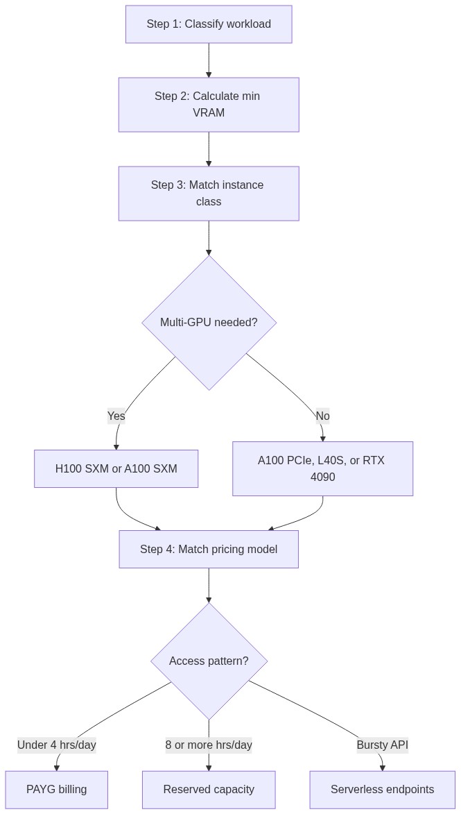
To walk this path with your own model, start with the VRAM number. Open a Python shell with your model config loaded and run sum(p.numel() for p in model.parameters()) * 2 / 1e9 to get the BF16 weight size in gigabytes. Add 20% for framework overhead and KV cache at moderate sequence lengths, then cross-reference the VRAM table above to find the smallest Runpod instance that clears it.
If you want to skip the base image setup entirely, Runpod Hub carries pre-built templates for vLLM, Axolotl (fine-tuning), and ComfyUI (diffusion) with CUDA, cuDNN, and library versions pre-configured for the target workload. A template gets you from VRAM calculation to a live inference endpoint in under 15 minutes. Validate your instance choice against real traffic before committing to reserved capacity.
Pick your model, run the calculation, and start building on Runpod with no waitlist and no sales call required.