Most teams swap out their OpenAI API key for a self-hosted endpoint and assume the hard part is over. Then production load arrives: latency spikes when three requests come in simultaneously, yet GPU utilization sits at 40% between bursts. The instinct is to add another GPU. But a card that’s only 40% busy under load doesn’t have a capacity problem, and a second one just gives you two half-idle GPUs and the same latency. The real question is why a GPU under load is only 40% busy in the first place.
The answer isn’t where most people look. It lives in the split between two fundamentally different compute phases, in how 60 to 80% of your VRAM gets silently wasted under naive memory allocation, and in batching behavior that either keeps your GPU busy or doesn’t. This guide traces a request from raw text through tokenization, through the inference loop, through the memory subsystem, and into a live serving endpoint, with every concept tied to a configuration decision you can make today.
LLM Inference: The Prefill/Decode Split
Inference is the process of running a trained model forward to produce output tokens given input tokens. It’s not fine-tuning, not training, not weight adjustment. The weights are frozen. You’re executing a fixed mathematical function billions of times, very fast.
That function doesn’t run as one atomic operation. It splits into two distinct phases with different performance characteristics.
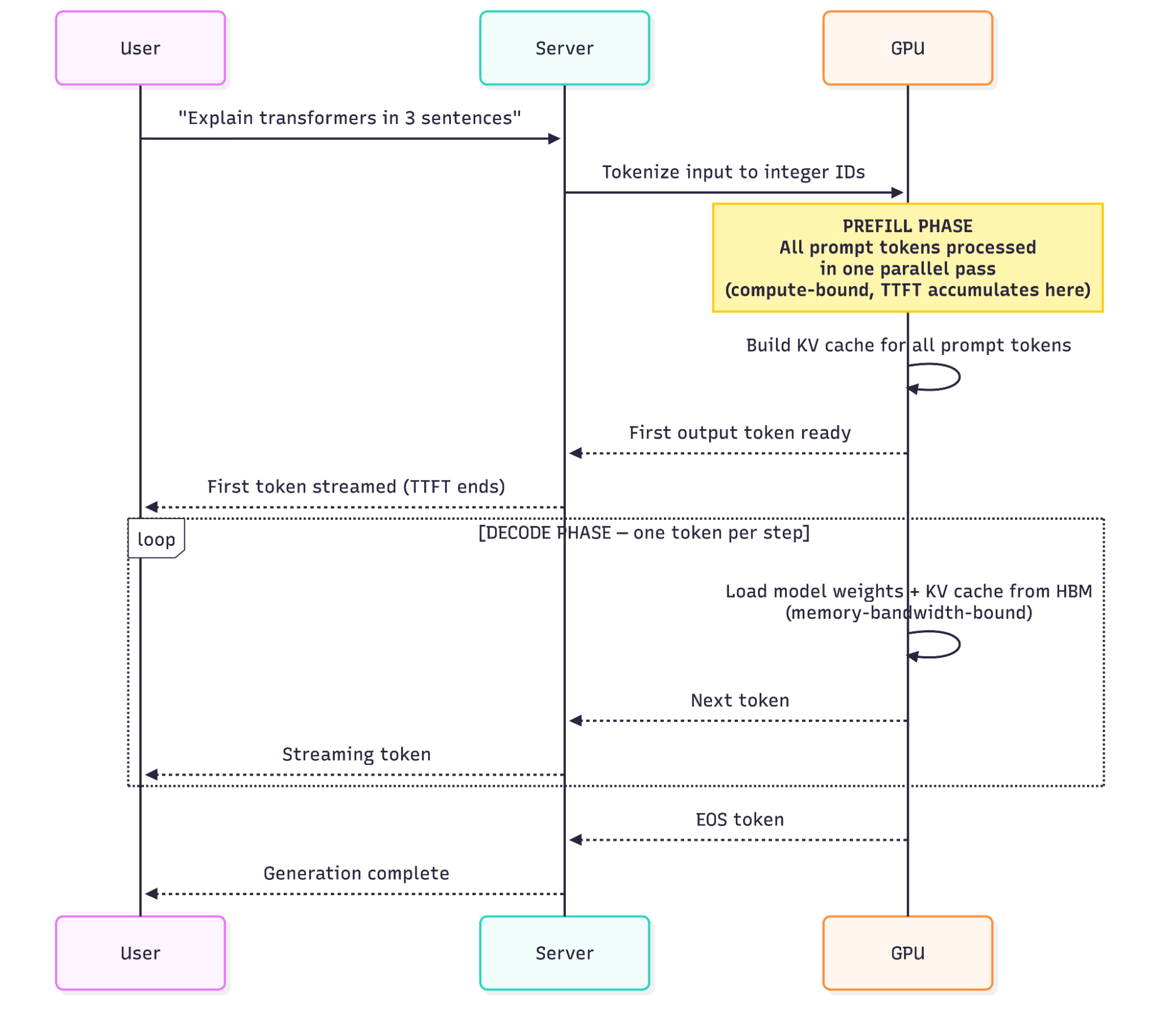
Prefill processes the entire input prompt in a single parallel forward pass. If your prompt is 512 tokens, the transformer’s attention mechanism operates on all 512 simultaneously, computing the query, key, and value tensors for every token at once. The phase is compute-bound: you’re doing a lot of matrix multiplication, and GPU FLOPS are the bottleneck. A longer prompt means a proportionally more expensive prefill. This is also where TTFT (time to first token) accumulates, since the user sees nothing until prefill completes.
Decode generates output tokens one at a time. Each forward pass produces exactly one new token, which gets appended to the sequence, and then you run another forward pass. Repeat until you hit a stop token or max_tokens. Decode is memory-bandwidth-bound: at each step, the GPU must load the full model weights (far too large to fit in on-chip SRAM) plus the growing KV cache from HBM (high-bandwidth memory) into the compute units. The actual matrix multiply is trivially fast; most of the step is spent waiting on data to arrive. Generating 500 tokens means 500 sequential forward passes, and there’s no way to parallelize across them.
The phase split matters for hardware selection and batching strategy. A GPU with high memory bandwidth will outperform a theoretically higher-FLOP card on single-request decode latency, because you’re not FLOP-limited in decode. You’re limited by how fast you can move data. The KV cache section returns to this with the specific bandwidth numbers and the hardware-evaluation conclusion.
The throughput-versus-latency tension follows directly from this structure. Serving one request at a time minimizes that request’s latency but wastes the GPU during decode gaps. Batching more requests together increases throughput but increases the wait time for each request’s first token. The rest of this guide is largely about managing that tradeoff.
Tokenization: What the Model Actually Sees
Before prefill can start, your raw text has to become integers. The model doesn’t process characters or words; it processes token IDs, which get looked up in a learned embedding table and converted to dense vectors that enter the first transformer layer. The embedding lookup is the first computation the model performs on your input, which is why token count, not character count, is the fundamental unit of cost, latency, and context capacity.
Most modern LLMs use Byte Pair Encoding (BPE) or a variant of it. BPE starts with individual bytes and iteratively merges the most common adjacent pairs into single tokens. The result is a vocabulary of 32,000 to 128,000 subword units covering common English words as single tokens, less common words as two or three tokens, and rare strings as many tokens. The word “tokenization” is a single token in some tokenizers and three tokens in others.
Three practical consequences follow from this.
Token count is not word count. A 2,000-word document typically runs 2,600 to 3,000 tokens, depending on content type and tokenizer. Code tokenizes efficiently for common patterns (keywords, standard identifiers) but less efficiently for unusual variable names. Non-Latin scripts (Chinese, Arabic, Japanese) often consume two to five times more tokens per unit of semantic content than English does, depending on the language and tokenizer. That token-density gap directly inflates both cost and latency for multilingual applications.
The context window is measured in tokens, not words. A 128K-token context window doesn’t hold 128K words. A developer passing in a full codebase should budget for roughly 1.3 to 1.5 tokens per word for English prose, and higher for mixed code-and-text inputs.
MAX_MODEL_LEN directly controls your VRAM bill. In Runpod’s vLLM deployment, this environment variable sets the maximum sequence length the engine allocates KV cache for. Set it too high and you’re pre-reserving VRAM that most requests will never use. Set it too low and requests exceeding the limit will be rejected with an error (or, if you have configured truncate_prompt_tokens, silently truncated, which leaves the model to process incomplete context without telling you). For a deployment where 95% of requests are under 4,096 tokens, setting MAX_MODEL_LEN=8192 instead of the model’s 128K default can free several GB of VRAM that PagedAttention can redirect toward concurrent request capacity.
Token count, context length, and VRAM allocation all feed directly into the metrics you’ll use to gauge whether your endpoint is performing well, which is where the next section picks up.
The Metrics Stack: What to Measure and Why
Three metrics cover the operational reality of LLM serving.
TTFT (Time to First Token) measures latency from request submission to the moment the first output token is received. It’s driven almost entirely by prefill duration, which scales with prompt length. A 100-token prompt might have a TTFT in the tens-of-milliseconds range on a warm endpoint. A 10,000-token prompt doing RAG document analysis might have a TTFT of one to several seconds on the same hardware, depending on GPU class and batch conditions. Interactive applications where users are watching a cursor blink are TTFT-sensitive; background batch jobs are not.
TPOT (Time Per Output Token) measures average decode latency per generated token. On a well-tuned vLLM endpoint serving an 8B model on an L40S, you’d expect roughly 15 to 25 ms per token under modest load, fast enough that streaming feels fluid. As concurrent request counts climb and the GPU saturates (for reasons the KV cache and serving-optimizations sections explain in detail), TPOT rises. Users perceive this as the stream slowing down mid-response.
Throughput is tokens generated per second across all concurrent requests, the cost-efficiency metric. If your endpoint generates 1,000 tokens per second at $0.60 per hour for the GPU, your cost per million output tokens is roughly $0.17. Double the throughput with better batching on the same hardware, and that cost drops to $0.085. This is why batching optimizations map directly to unit economics.
The latency-throughput tradeoff is concrete. When you batch 10 requests together instead of processing them sequentially, GPU utilization improves and throughput climbs, but every request in that batch waits until the batch is assembled before its prefill starts. For a chat application, that wait is perceptible. For an offline data enrichment pipeline running 50,000 API calls overnight, it’s irrelevant.
Choosing the right metric to optimize isn’t a technical question. It’s a product question. Know your workload shape before you tune. What constrains all three metrics on the same GPU is primarily memory, which is where the next section begins.
Memory Is the Bottleneck: KV Cache and PagedAttention
Each decode step reuses the key and value tensors computed during prefill and accumulated during prior decode steps. Without caching, every decode step would reprocess the full sequence from scratch, a cost that grows quadratically with sequence length. The KV cache stores those tensors so each step only has to compute the new token’s attention contribution.
The KV cache is expensive. For a 7B-parameter model using grouped-query attention (GQA) in BF16 at a sequence length of 4,096 tokens, as with Llama 3.1 8B Instruct, each request’s KV cache consumes roughly 512 MB. Older 7B models using multi-head attention (32 KV heads) produce closer to 2 GB per request at the same sequence length, so the figure is architecture-specific. With a 40 GB A100, that leaves roughly 26 GB after model weights (~14 GB) are loaded, supporting about 50 simultaneously cached sequences at 512 MB each, assuming zero fragmentation.
Naive allocation produces extreme waste. The classical approach pre-allocates a contiguous memory block sized to max_sequence_length for every request the moment it arrives. A request asking for a 100-token output tied to a 4,096-token context gets the same allocation as one that will actually use 4,000 tokens. Since most requests don’t fill their allocated slot, Woosuk Kwon et al.’s 2023 SOSP paper on vLLM measured memory fragmentation at 60 to 80% under typical workloads. On a 40 GB A100 with 60% waste in the KV cache budget (~26 GB after weights), you’re effectively operating with around 10 GB of usable KV cache capacity. At 512 MB per request, that’s roughly 20 concurrent sequences, less than half the 50 you’d get under zero-fragmentation accounting. Concurrency limits immediately.
PagedAttention solves this by borrowing the operating system’s virtual memory model. Instead of one contiguous block per request, KV cache is divided into fixed-size physical blocks, 16 tokens per block by default in vLLM (verify against your deployed version, as this default has shifted across major releases). A block is only allocated when it’s actually needed. When a request generates its 17th token, a second block is allocated. When the request finishes, those blocks are immediately freed and available for new requests.
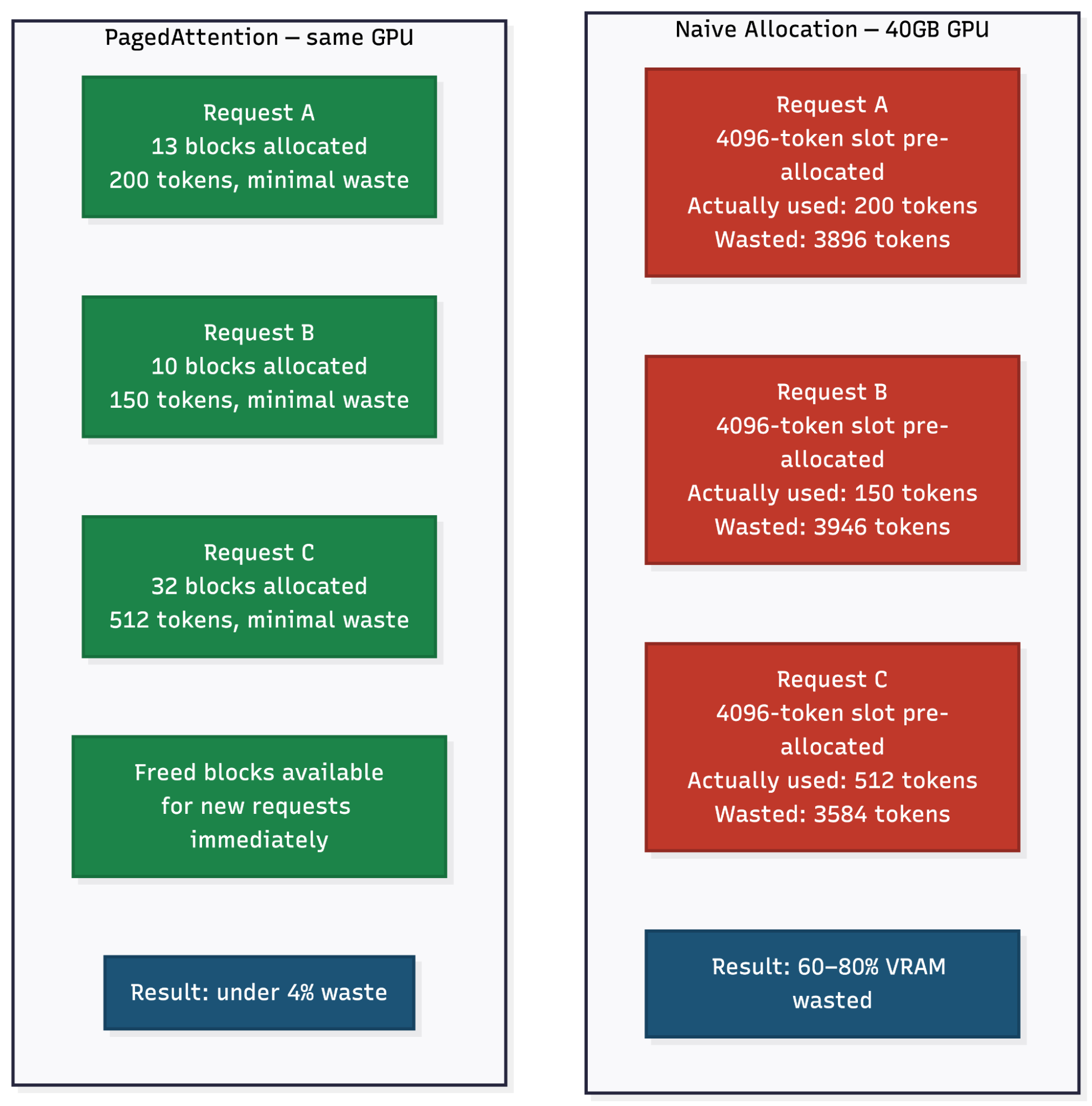
Kwon et al. measured memory waste falling from 60 to 80% under naive allocation to under 4% with PagedAttention. On the same hardware, that reduction in waste translates directly to more concurrent requests and higher throughput.
In Runpod’s vLLM deployment, GPU_MEMORY_UTILIZATION controls how much of the available VRAM is committed to the KV cache pool. Setting it to 0.90 tells vLLM to reserve 90% of GPU memory for model weights plus KV blocks, leaving 10% for overhead. Setting it to 0.95 squeezes out more concurrent capacity but leaves less headroom for unexpected spikes. A common starting point is 0.90 (the current vLLM default is 0.92); adjust upward or downward based on observed OOM behavior for your specific workload.
One more point on memory bandwidth. When vLLM processes a decode step, it loads model weights and KV cache from GPU HBM, runs a small matrix multiply, and writes results back. The compute is trivial; the data movement is slow. An H100 SXM’s 3.35 TB/s HBM3 bandwidth is not a marketing number. It directly determines how fast you can stream tokens on single-request workloads. This is why memory bandwidth specs matter more than theoretical TFLOPS when you’re evaluating hardware for inference.
With the memory subsystem understood, the next question is how to make the best use of the capacity it provides, through batching, quantization, and decode-phase acceleration.
Serving Optimizations: The Levers That Matter
Three levers account for most of the throughput and latency you can recover on a fixed GPU budget: continuous batching, quantization, and speculative decoding. The first keeps the GPU saturated under concurrent load, the second cuts the memory and bandwidth cost of the weights, and the third attacks decode latency directly. Continuous batching delivers the largest payoff for most serving workloads, so start there.
Continuous Batching
Static batching waits for a full batch to assemble, runs all requests together, and releases the batch when every request finishes generating. The problem: requests finish at different times. If one request in a 16-request batch generates 50 tokens and the others generate 500, the GPU sits waiting on the slow requests while the finished slot goes empty.
Continuous batching inserts new requests into the active batch as soon as slots free up. A request that finishes after 50 tokens immediately opens its slot for a queued request, with no waiting for the rest of the batch to complete. The GPU stays saturated rather than cycling through idle periods.
vLLM implements continuous batching by default. MAX_NUM_SEQS controls the upper bound on concurrent sequences in the active batch. Setting it to 256 means vLLM will accept up to 256 requests into the active batch, but actual concurrency is also gated by available KV cache blocks. On a GPU where the KV cache pool supports only 50 concurrent sequences at your typical sequence length, MAX_NUM_SEQS=256 won’t materially increase throughput beyond that limit. Start with MAX_NUM_SEQS at or slightly above the KV-cache-derived concurrency ceiling you calculated from GPU_MEMORY_UTILIZATION and MAX_MODEL_LEN.
Runpod’s vendor benchmarks compare against HuggingFace Transformers’ single-request vanilla generation loop, a deliberately conservative reference baseline, and report throughput improvements of 24x. Independent results will vary by model size, GPU, and traffic pattern. Text Generation Inference (TGI) introduced its own continuous batching support in late 2023, so direct comparisons against TGI should account for that, since it significantly narrows any earlier throughput gap. The directional improvement from continuous over static batching is well-established across the literature.
Quantization
Quantization reduces the numerical precision of model weights, which cuts VRAM requirements and increases the rate at which the GPU can move data through its memory bus.
The progression: FP32 (4 bytes/param) → BF16 (2 bytes/param) → INT8 (1 byte/param) → INT4 (0.5 bytes/param). A 7B-parameter model in FP32 requires about 28 GB. In BF16 it’s about 14 GB. In INT4 it’s about 3.5 GB. Quality degradation is not linear. BF16 is generally equivalent to FP32 for standard inference workloads, INT8 with careful calibration is often imperceptible, and INT4 shows degradation on reasoning-heavy tasks that is sometimes acceptable and sometimes not. Verify on your specific model and task before committing to production.
BF16 is the practical default. In Runpod’s vLLM configuration, DTYPE=bfloat16 sets this. It delivers full-precision-equivalent inference at half the VRAM of FP32, with native hardware support on Ampere (A100) and Hopper (H100) GPUs. Dropping to INT8 or INT4 is worth benchmarking if you’re VRAM-constrained and the quality tradeoff is acceptable, but verify on your specific model and task before committing to production.
Speculative Decoding
Speculative decoding uses a small, fast draft model to generate several candidate tokens in a single step, then uses the full target model to verify them in parallel. Since verification is cheaper than generating each token independently, accepted tokens arrive at lower latency than sequential decode. It works best for predictable outputs (structured code generation, templated responses) where the draft model guesses correctly most of the time. vLLM supports speculative decoding as a documented configuration option with multiple methods including draft models, EAGLE, and N-gram. It’s worth knowing it exists. It’s not the first optimization to reach for.
Once the optimization levers are understood, the remaining question is where to run the workload, which determines the economics and operational model.
Serving Architectures: Serverless vs. Dedicated
The serving architecture decision comes down to traffic pattern and cost math.
Serverless endpoints scale from zero to N replicas based on incoming request volume and charge per second of compute consumed. You pay only while requests are being processed. For variable or bursty traffic, a startup that sees 10 requests per hour most of the time but spikes to 500 per hour during business hours, serverless means you’re not paying for idle GPU capacity during the quiet periods.
Runpod’s Serverless platform runs vLLM natively and exposes the configuration knobs covered in this guide as first-class environment variables, not hidden defaults. Cold start behavior depends on your model deployment strategy. With cached models (the simpler path), Runpod attempts to start workers on hosts that already have the model downloaded. No Docker build is required, but cold starts on uncached hosts incur the full model download latency. Runpod’s FlashBoot optimization significantly reduces cold-start latency for serverless workers, though startup time still scales with model size. With baked-in models, you build a custom Docker image with weights included, eliminating the download step and reducing cold start variance to just container initialization time. For latency-sensitive deployments where cold-start variance is unacceptable, baked-in weights are the right call.
Dedicated GPU pods provide a persistent instance with no cold start and full environment control. You select specific hardware (A100 80GB, L40S, H100) and the instance runs until you terminate it. The per-hour rate is fixed regardless of whether you’re serving 1 request or 1,000 per hour. This makes dedicated pods economically efficient once sustained request volume is high enough that per-second billing would exceed the reserved hourly rate. To calculate the crossover: pull the per-second rate for your GPU tier from Runpod Serverless pricing and the reserved hourly rate from Runpod’s GPU pricing, then multiply your projected monthly active GPU-seconds against both billing models. Switch to dedicated when the reserved hourly rate is cheaper over your expected utilization window.
Tensor parallelism splits model weights across multiple GPUs using the TENSOR_PARALLEL_SIZE environment variable. Set TENSOR_PARALLEL_SIZE=2 to split across two GPUs, TENSOR_PARALLEL_SIZE=4 across four. This is the only practical path for models that exceed a single GPU’s VRAM. A 70B-parameter model in BF16 requires about 140 GB, which exceeds even an H100 SXM’s 80 GB. On Runpod, select a multi-GPU pod SKU (see the full GPU catalog) and set TENSOR_PARALLEL_SIZE to match the GPU count. Tensor parallelism adds inter-GPU communication overhead that increases TPOT; splitting across two GPUs doesn’t double throughput, but it makes large models physically possible.
The serverless and dedicated paths above map directly to the two deployment walkthroughs that follow.
Production Deployment: Your First vLLM Endpoint on Runpod
Two paths get you from zero to a live, OpenAI-compatible endpoint.
Path A: Serverless (Recommended Starting Point)
This takes under 10 minutes and costs nothing until a request hits the endpoint.
- Log in to the Runpod console and navigate to the Serverless tab.
- Under “Quick Deploy,” select the Serverless vLLM card and click Start.
- Enter your model name, for example meta-llama/Llama-3.2-3B-Instruct. For gated Hugging Face models, add HF_TOKEN in the environment variables section.
- Click Next and select your GPU type. An L4 or RTX 4090 handles a 3B model comfortably. A 70B model needs an A100 80GB or equivalent for quantized (INT4/INT8) inference; full-precision (FP16/BF16) deployment requires multiple GPUs with tensor parallelism.
- Click Advanced to set MAX_MODEL_LEN (for example, 8192) and GPU_MEMORY_UTILIZATION (for example, 0.90). Leave MAX_NUM_SEQS at the default for your first deployment; tune it under real load once you have baseline TTFT and throughput measurements.
- Click Deploy.
Monitor the Logs tab. You’re waiting for INFO: Application startup complete. Two common failure patterns to watch for: CUDA out of memory during weight loading (the selected GPU doesn’t have enough VRAM for the model in the chosen dtype, so switch to a larger GPU or reduce DTYPE to bfloat16 if it isn’t already), and model download stalls or failures (verify HF_TOKEN is set for gated models, or check Hugging Face’s status page if download progress freezes unexpectedly). Once startup completes, the endpoint is live. Use the Requests tab to send a test completion directly in the console, no additional tooling required.
The endpoint is OpenAI-compatible. Swap it into any existing OpenAI client by changing the base URL and API key:
No re-architecture required. Any code that already calls OpenAI’s API works as-is.
Serverless covers most teams’ starting needs. The second path matters once traffic patterns shift toward sustained load or your deployment needs container-level control that Serverless’s managed model doesn’t expose.
Path B: GPU Pod (For Sustained Load or Custom Environments)
Use this path for teams that need persistent infrastructure, full environment control, or sustained request volumes where reserved capacity beats per-second billing.
- Spin up an L40S or A100 80GB GPU pod using a pinned vLLM image tag rather than latest (for example, vllm/vllm-openai:v0.8.5; replace with the current stable release from the vLLM releases page). Using latest means a container restart can silently pull a breaking version.
- Attach a Network Volume and configure the mount path to /root/.cache/huggingface for model weight caching across restarts. Runpod volumes require an explicit mount path during pod creation.
- Expose port 8000.
- Set the container start command:
Generate an API key from Account → Settings → API Keys in the Runpod dashboard before deploying. vLLM defaults to binding 127.0.0.1, so pass --host 0.0.0.0 explicitly in Docker or pod environments that need external access. The server accepts OpenAI-format requests from the moment vLLM finishes loading weights.
For production monitoring, vLLM exposes Prometheus metrics at /metrics on its serving port (default 8000), no additional vLLM configuration required. Point your Prometheus scrape config at http://<pod-ip>:8000/metrics. Track vllm:e2e_request_latency_seconds for TTFT distribution, vllm:generation_tokens_total for throughput, and GPU utilization via DCGM metrics. Watch for high GPU memory utilization combined with low GPU compute utilization. That pattern usually means KV cache pressure is forcing vLLM to wait on memory rather than compute, often a sign that MAX_MODEL_LEN is set higher than your actual workload demands, or that GPU_MEMORY_UTILIZATION needs adjustment.
Conclusion: From Concept to Configuration
The gap between “calls the API” and “understands the inference engine” is exactly where performance and cost decisions get made. Decode is memory-bandwidth-bound, which is why you’re evaluating HBM bandwidth and not TFLOPS. PagedAttention’s reduction of VRAM waste from 60 to 80% down to under 4% is what GPU_MEMORY_UTILIZATION=0.90 actually controls. MAX_NUM_SEQS is the lever for batch concurrency, and tuning it changes throughput in ways that adding GPU count alone cannot.
Runpod’s vLLM Serverless endpoints expose these knobs directly as environment variables, not as opaque defaults or infrastructure decisions someone else made for you. Pick a model you already know from Hugging Face, deploy Path A using the Serverless vLLM Quick Deploy flow, and send a test completion through the Requests tab. With scale-to-zero, you pay nothing until a worker spins up to handle your first request.
A first-deployment configuration checklist worth keeping at hand:
- Pick a model that fits your target GPU’s VRAM in your chosen dtype (BF16 for most cases).
- Set MAX_MODEL_LEN to your real p95 sequence length, not the model’s default. Pre-reserving 128K of KV cache when 95% of requests stay under 4K wastes most of your GPU.
- Start with GPU_MEMORY_UTILIZATION=0.90 and adjust based on observed OOM behavior under load.
- Leave MAX_NUM_SEQS at default for the first deployment; tune it once you have baseline TTFT and throughput data.
- For Serverless, use Quick Deploy. For Pods, pin a specific vLLM image tag rather than latest.
- Wire Prometheus to /metrics on port 8000 from day one so TTFT and throughput are visible before you need them.
Related guides
Author profile: Damaso Sanoja